This webpage is intended to explain why the DMRG algorithm is equivalent to the singular-value-decomposition (SVD) using more mathematical languages. First, what is SVD? SVD is a generalized decomposition for a \( M \times N\) rectangle matrix, written as
where \( \widehat{U} \) has dimension of \( M \times \min(M,N)\), composed of orthonormal columns and \( \widehat{U}^{\dagger}\widehat{U}=I\); if \( M \le N\), we also have \( \widehat{U}\widehat{U}^{\dagger}=I\); \( \widehat{V}^{\dagger} \) has dimension of \( \min(M,N) \times N \), composed of orthonormal rows and \( \widehat{V}^{\dagger} \widehat{V}=I\); if \( M \ge N\), we also have \( \widehat{V}\widehat{V}^{\dagger}=I\). \( D \) is a \( \min(M,N) \times \min(M,N)\) non-negative diagonal matrix, whose elements are called singular values. We usually use the descending order convention: \( s_1 \ge s_2 \ge s_3 \ge \cdots \ge s_r\), where \( r = \min(M,N) \).
Suppose now we are looking for \( r^{\prime} < r\), such that
where \( \widehat{\bar{D}}\) has \( s_1 \ge s_2 \ge s_{r^{\prime}} \ge 0 \cdots\), and \( \widehat{\bar{U}} \) has dimension of \( M \times r^{\prime} \) and \( \widehat{\bar{V}}^{\dagger} \) has \( r^{\prime} \times N \). \( \widehat{\bar{A}} \) is truncated with rank \( r^{\prime} < r \). Linear Algebra tells us that the above SVD process provides a solution to minimize \( \lvert \widehat{A} - \widehat{\bar{A}} \lvert ^2 \), i.e. \( \widehat{\bar{A}} \) is the approximate matrix (with lower rank) to best describe \( \widehat{A} \).
So, what is the relation between DMRG and SVD? Suppose now we have a system which can be described in terms of two subsystems, left and right blocks. Any wave function can be written as
\begin{equation*}
\lvert \Psi \rangle = \sum_{L,R} \psi_{L,R} \lvert L \rangle \lvert R \rangle,
\end{equation*}
where \(\sum^M_{L=1} \lvert L \rangle \langle L \lvert = I\) and \(\sum^N_{R=1} \lvert R \rangle \langle R \lvert = I\) form the complete sets for the left and right blocks. The reduced density matrix for the \( L \) and \( R \) blocks are separately defined as
The \(\textrm{Tr}_R \) means the partial trace over \( R \) block, i.e. \(\textrm{Tr}_R = \sum_R \langle R \lvert \cdots \lvert R \rangle \). Hence the density matrix of the \( L \) block is
\begin{equation*}
\widehat{\rho}_L \lvert a \rangle = w_a \lvert a \rangle.
\end{equation*}
The value of \( w_a \) has a physical meaning, the probability of the state \( \lvert a \rangle \) existing in the system \( \lvert \Psi \rangle \), and we have \( \sum^M_{a=1} w_a =1 \). Next we truncate the degrees of freedom. We choose \( \lbrace \lvert a \rangle \rbrace \) with \( r^{\prime} \) largest eigenvalues \( w_a, a=1,\cdots r^{\prime} \) (\( r^{\prime}< M \)) to construct the transformation matrix, shown as \( U_{La} = \langle L \lvert a \rangle \) and the relation between the new states and old ones is \( \lvert a \rangle =\sum_L \langle L \lvert a \rangle \lvert L \rangle = \sum_L U_{La} \lvert L \rangle\). Such a selection maximizes \( \sum^{r^{\prime}}_{a=1} w_a \).
To be more concise, we can use matrix representation for the above procedures. Suppose the degrees of freedom of the \( L \) and \( R \) block are \( M \) and \( N \), we can write the wave function as a \( M \times N \) matrix \( \widehat{\Psi} \). The \( \widehat{\Psi} \) matrix can be SVD as
Then the \( L \) block density matrix is \( \widehat{\rho}_L = \widehat{\Psi} \widehat{\Psi}^{\dagger} \) and the \( R \) one \( \widehat{\rho}_R = \widehat{\Psi}^{\dagger} \widehat{\Psi} \). Plugging the above decomposition into \( \rho_{L,R} \), we have
\begin{equation*}
\widehat{\rho}_L = \widehat{U} \widehat{D}^2 \widehat{U}^{\dagger}, \ \widehat{\rho}_R = \widehat{V} \widehat{D}^2 \widehat{V}^{\dagger}.
\end{equation*}
By diagonalizing the density matrices, we naturally obtain \( \widehat{U} \) and \( \widehat{V} \), and the matrix element of \( D^2 \) satisfies \( s^2_a = w_a \). The density matrix renormalization scheme is equivalent to the SVD process.
On the other hand, recalled that the basis state transformations are represented as \( \lvert a \rangle= \sum _L U_{La} \lvert L \rangle \) and \( \lvert b \rangle= \sum_R V_{Rb} \lvert R \rangle \) for the \( L,R \) blocks, separately. Note that such a convention is used for the renormalization process to add one site into a block. For example, if \( \lvert L,R \rangle \) are the quantum states for the \( k \)-sites blocks, then \( \lvert a,b \rangle \) denote the quantum states for the block with \( k+1 \) sites.
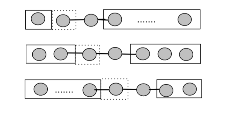
However, in the DMRG sweep algorithm, when the \( L \) block enlarges, the \( R \) block shrinks, vice versa; i.e. for \( L \), \( k \to k+1 \), but for \( R \), \( l \to l-1 \). The schematic is shown on the right. Thus, to be more clear, we should label \( \lvert a \rangle_{k+1} = \sum_L U_{La} \lvert L \rangle_k \) and \( \lvert b \rangle_{l+1}= \sum_R V_{Rb} \lvert R \rangle_l \). This means the number of sites \( \sim k+l \) keeps fixed. The transformation on the \( R \) block can be further rewritten as \( \lvert b \rangle_{l-1}= \sum_R V^{*}_{Rb} \lvert R \rangle_l \).
Combined these, we have
\begin{equation*}
\lvert \Psi \rangle = \sum_{L,R} \psi_{L,R} \lvert L \rangle \lvert R \rangle = \sum_{L,R} \sum_a U_{La}D_{aa}V^*_{Ra} \lvert L \rangle \lvert R \rangle = \sum_a s_{a} \Big( \sum_L U_{La} \lvert L \rangle \Big) \Big( \sum_R V^*_{Ra} \lvert R \rangle \Big),
\end{equation*}
\begin{equation*}
\lvert \Psi \rangle = \sum^r_{a=1} s_a \lvert a\rangle_L \lvert a \rangle_R.
\end{equation*}
The subscripts emphasizes \( L,R \) blocks. \( \lbrace \lvert a\rangle_L \rbrace \) and \( \lbrace \lvert a\rangle_R \rbrace \) form the orthonormal sets for block \( L,R \). The last step generates the so-called Schmidt decomposition. With truncation, i.e. choosing \( r^{\prime} < r \), the Schmidt decomposition gives the approximated wave function