As we mentioned, the numerical techniques, Markov-chain Monte Carlo (MCMC), Dynamical mean field theory (DMFT) and Density matrix renormalization groups (DMRG) have connection to the machine learning algorithms in data science. In short, these computational methods are designed to reduce the dimension of state space to solve large degrees-of-freedom complex problems.
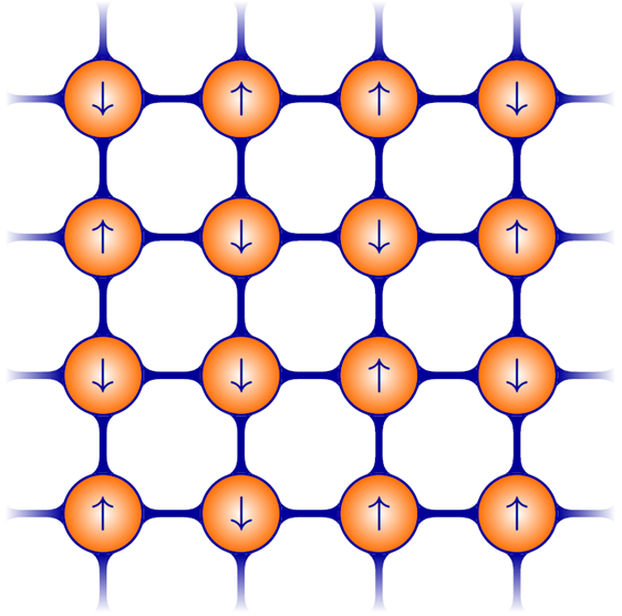
What do "large degrees-of-freedom" and "complex" explicitly mean? Let me explain it further. Suppose now we have a lattice, and on each lattice unit, we load an electron. The electrons are localized on the units and carry spin, either spin-up or spin-down, the quantum state labeled as \( \lvert 0 \rangle \) and \( \lvert 1 \rangle \). The figure below shows an example on a \( 4 \times 4 \) square lattice, with 16 units. The spin states \( \uparrow \) and \( \downarrow \) can be translated to \( \lvert 0 \rangle \) and \( \lvert 1 \rangle \). To identify the local state, we can design an measurement, such that \( S^z \lvert \uparrow,\downarrow \rangle = s \lvert \uparrow, \downarrow \rangle \); \(s = + (-) \) means \( \uparrow (\downarrow) \) spin. In machine learning community, this system corresponds to Markov random fields for image denosing, as well as the Restricted Boltzmann Machine for collaborative filtering.
In a little more professional language, we say the state space of each unit has
\( q \ (\textrm{degrees of freedom}) = 2 \), since the quantum state can be
\( \lvert 0\rangle \) or
\( \lvert 1 \rangle \). If there are two units,
\( q=2^2 \), since
\( \lvert 00 \rangle \),
\( \lvert 01\rangle \),
\( \lvert 10\rangle \) and
\( \lvert 11\rangle \). Next let us further consider the system is an one-dimensional chain with 4 units. The degrees of freedom of the entire system becomes
\( D= q^4 = 2^4 =16 \). The possible configurations are
\( \lvert 0000\rangle \),
\( \lvert 0001\rangle \),
\( \lvert 0010\rangle \),
\( \cdots \lvert 1111\rangle \). If the system is a
\( 4 \times 4 \) square lattice (like the left figure) in two dimensions, there are
\( D= 2^{16}= 65536 \) configurations. These symbols
\( \lvert \cdots \rangle \) are nothing but the bits in computers; the number of units is the number of bits of a computer. In this (classical) Boltzmann machine, the system is explicitly in one of possible configurations, say either
\( \lvert 0000\rangle \) or
\( \lvert 0001\rangle \) or
\( \cdots \lvert 1111\rangle \) (like the
Schrödinger's cat is either alive or dead.).
The concept in quantum mechanics goes beyond the classical picture. In quantum mechanics, we allow the system state be "linear combination" of the configurations, i.e.
\begin{equation*}
\lvert \Psi \rangle = \phi_0 \lvert 0000 \rangle + \phi_1 \lvert 0001 \rangle + \cdots + \phi_{15} \lvert 1111 \rangle.
\end{equation*}
\( \lvert \Psi \rangle \) is called the wave function. The system is not specifically being
\( \lvert 0001\rangle \) or
\( \lvert 1111 \rangle \), but it has probability
\( \lvert \phi_0 \lvert^2 \) being
\( \lvert 0000\rangle \),
\( \lvert \phi_1 \lvert^2 \) being
\( \lvert 0001\rangle \) and probability
\( \lvert \phi_{15} \lvert^2 \) being
\( \lvert 1111\rangle \) (if the coefficients are normalized, then
\( \sum_i \lvert \phi_i \lvert^2 =1 \)). In other words, the system could be
\( \lvert 0000\rangle \) "and"
\( \lvert 0001\rangle \cdots \) "and"
\( \lvert 1111 \rangle \) (now we say the Schrödinger's cat has some possibility to be alive and be dead.). As long as the existing probability is nonzero, the system has chance to be any configurations. In all, in the quantum mechanics world, it is not deterministic; probability dominates.
Hence, to solve the wave functions, we need to know the equation of motion, or called Hamiltonian matrix, and diagonalize to find the eigenstate, or the wave function. The difficulty to solve the eigen-problems depends on whether the matrix is diagonal or off-diagonal. As the interaction between two spins is a diagonal type, the model is in the classical manner. As an example, the diagonal interaction of the binary model (\( q=2 \)) we described above is
\begin{equation*}
H = \sum_{(i,j) \in \textrm{bond}} J_{ij} S^z_i S^z_j + \sum_i h_i S^z_i,
\end{equation*}
such that
\( \big( J_{ij} S^z_i S^z_j +h_iS^z_i+h_j S^z_j \big) \lvert s_i s_j \rangle = \big( J_{ij} s_i s_j +h_is_i +h_j s_j \big) \lvert s_i s_j \rangle \). We see that the input state is the same as the output state up a constant, i.e.
\( \lvert s_i s_j \rangle \to \big( J_{ij}s_is_j + \cdots \big)\lvert s_i s_j \rangle \) where
\( \big( J_{ij}s_is_j + \cdots \big) \) is just a number. Hence we always have
\( H \lvert s_1 s_2\cdots s_N \rangle = E \lvert s_1 s_2\cdots s_N \rangle \), where
\( E \) is a number. This is the well-known
Ising model. This model is used to simulate classical magnetic phenomena in thermal physics.
On the other hand, the off-diagonal type of the binary model reads as
\begin{equation*}
H = \sum_{(i,j) \in \textrm{bond}} J_{ij} S^z_i S^z_j + \sum_{(i,j) \in \textrm{bond}} J_{ij} S^x_i S^x_j+ \sum_i h_i S^y_i,
\end{equation*}
where the pairwise terms
\( S^x_i S^x_j \) and the onsite field
\( S^y_i \) bring the off-diagonal matrix elements in the Hamiltonian matrix; i.e.
\( S^x_i S^x_j \lvert \uparrow \downarrow \rangle \sim b\lvert \downarrow \uparrow\rangle \) and
\( S^y_i \lvert \uparrow \rangle \sim c \lvert \downarrow \rangle \), where
\( b,c \) are some numbers. Now we can see that the input state is different from the output state. The physical meaning here is that
\( S^x_i S^x_j \) will flip the spin on site-
\( i \) and site-
\( j \) simultaneously. This makes all spins
correlated and the system is in the quantum manner. This model is called
Heisenberg model, a quantum version of the Ising model, used to describe magnetic systems at very low temperatures.
Another concern about the problem is that the dimension of the Hamiltonian matrix exponentially grows up. The example binary model has \( 2^N \) possible states. As \( N \sim 100 \), diagonalizing a \( 2^{100}\times 2^{100} \) matrix becomes impossible. However, the situation could be even worse. For many purposes, we need to remodel the system to allow electrons move, with more configurations or space states for each lattice site; as in the Hubbard model, in addition to the quantum state labeled as \( \lvert \uparrow \rangle \) and \( \lvert \downarrow \rangle \) (single electron), we have \( \lvert \emptyset \rangle \) (no electron exists) and \( \lvert \uparrow\downarrow \rangle \) (two electrons exist on the same site) on each site. Therefore, the state space on each site is \( q=4 \) and the total degrees of freedom is \( D = 4^N \).
Therefore, solving the complex systems with blooming degrees of freedom is a challenge. In physics, we established a variety of numerical methods to approximately solve the problems: either performing dimensionality reduction or finding the effective models. This is similar to the spirit in data science. In the followings, I will explain the algorithms (try without using too much terminology) and show the implementation in machine learning.
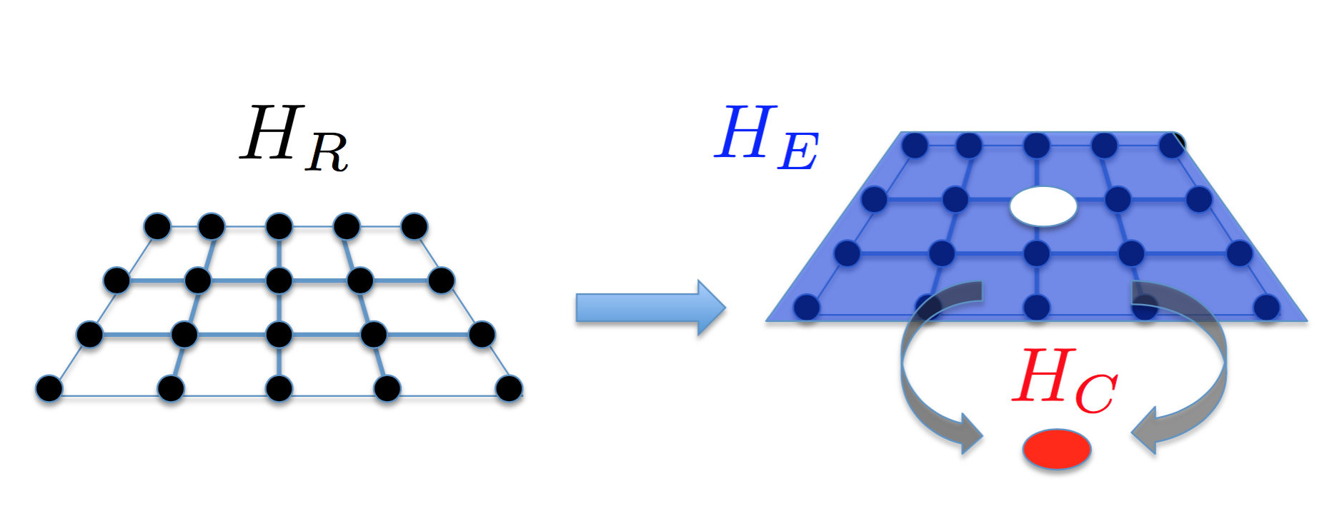
DMFT is a numerical recursive method to build effective models which can approximately describe complex systems. The entire system is mapped into a cluster \( C \) coupled to the environment \( E \). Such a mapping turns out to be exact in infinite dimensions. In 3D oxide materials, this approach has been shown to be a good approximation.
Suppose we are solving a real-world system described by \( H_R \); then in DMFT our goal is to find out \( H_C \) and \( H_E \), such that
\begin{equation*}
H_R \to H_C(\alpha_1, \alpha_2, \cdots) + H_E(\beta_1, \beta_2, \cdots) +H_{CE}(\gamma_1, \gamma_2, \cdots),
\end{equation*}
where
\( H_C(\alpha_1, \alpha_2, \cdots) \) and
\( H_E(\beta_1, \beta_2, \cdots) \) describe the effective equations of motion (remember, we called it Hamiltonian in physics) of the cluster and the environment, respectively;
\( H_{CE}(\gamma_1, \gamma_2, \cdots) \) represents coupling (interaction) between the cluster
\( C \) and the environment
\( E \). The right hand side is the approximate model we are looking for.
The model parameters \( \lbrace \alpha_i, \beta_i, \gamma_i, \cdots \rbrace \) are needed to be determined numerically, such that the left hand side and right hand side have similar physical response and behavior. In physics, we use the so-called Green function to judge the "similarity" criterion. Given a set of \( \lbrace \alpha_i, \beta_i, \gamma_i, \cdots \rbrace \), we solve the cluster Green fucntion \( G_{C} \) of the \( H_C+H_E+H_{CE}\). With the cluster Green function, we can find the self-energy, and use the self-energy to generate the lattice Green function \( G_{lat} \) ("lat" meaning a real-world system without interaction which can be easily solved, but with some corrections). Once the lattice Green function is found, we minimize the following
\begin{equation*}
\chi = \sum_{i\omega_n} \Big| \Big( i\omega_n + \sum_i \widetilde{\alpha}_i - \sum_i \frac{\lvert \widetilde{\gamma}_i\lvert ^2}{(i\omega_n-\tilde{\beta}_i)} \Big) -G_{lat}(i\omega_n) \Big|^2
\end{equation*}
to fit the parameters
\( \lbrace \widetilde{\alpha}_i, \widetilde{\beta}_i, \widetilde{\gamma}_i \rbrace \) and go back to compute
\( G_{C} \). Iteratively do the above procedures, until the cluster Green function
\( G_{C} \) is approximate to the lattice Green function
\( G_{lat} \)
\begin{equation*}
G_C(i\omega_n) \approx G_{lat}\big[ i\omega_n, G_C(i\omega_n)\big], \ \textrm{for each} \ \omega_n
\end{equation*}
or equalivently
\( \lbrace \widetilde{\alpha}_i, \widetilde{\beta}_i, \widetilde{\gamma}_i\rbrace \approx \lbrace \alpha_i, \beta_i, \gamma_i\rbrace\), then "physically"
\( H_{R} \sim H_C+H_E+H_{CE}\). (Note here we used "physically" rather than "same", since they have different dimensions.)
We use the conjugate gradient to perform the least square fitting, i.e. \( \min_{\lbrace \alpha,\beta, \cdots\rbrace} \chi \) to find \(\lbrace \alpha_i, \beta_i, \gamma_i\rbrace\). Once \( \lbrace \alpha_i, \beta_i, \gamma_i, \cdots \rbrace \) are known, we have built an effective model ready for further predictions. This part of the DMFT algorithm is the same as linear regression. In simple linear regression, the cost function is defined as
\begin{equation*}
\chi = \Big| h_{\Theta}(X) - Y \Big|^2,
\end{equation*}
where
\( h_{\Theta} (X)=\theta_0 + \theta_1 x_1 +\theta_2 x_2 +\cdots \) is the hypothesis;
\( \Theta = \lbrace \theta_0, \theta_1, \cdots \rbrace \) are coefficients needed to be determined. By comparison, the hypothesis in the DMFT is defined as
\begin{equation*}
h_{\Theta} = i\omega_n + \sum_i \tilde{\alpha}_i - \sum_i \frac{\lvert \tilde{\gamma}_i\lvert ^2}{(i\omega_n-\tilde{\beta}_i)},
\end{equation*}
Hence the DMFT algorithm is to resursively performing regression, and then use the convergent results of
\( \Theta = \lbrace \alpha, \beta, \gamma,\cdots \rbrace \) to determine the effective predictive models. This concept is similar to data science.
DMRG is designed to solve 1D complex nanomaterials. Similarly, in 1D we have to face exponential degrees of freedom, and our goal is to find representative states (with m degrees of freedom) to approximately describe the true system (with \( D \gg m\) degrees of freedom)
\begin{equation*}
\sum^m_{i=1} \bar{\phi}_i \lvert \bar{a}_i \rangle \approx \sum^{D}_{i=1} \phi_i \lvert a_i \rangle
\end{equation*}
By iteratively performing singular-value-decomposition on the quantum states of a system, the approximated
\(\bar{\phi}_i\) and
\(\lvert \bar{a}_i \rangle \) are accessible. In this case we reduce system dimensionality and complexity (from
\(\infty \) to finite
m), called numerical renormalization process. In the DMRG algorithm, the renormalization process implements
\( m \) high-weighted eigenstates of the density matrix to represent
\( \lvert \bar{a}_i \rangle \), to minimize
\( \ \chi = \big| \sum \phi_i \lvert a_i \rangle - \sum \bar{\phi}_i \lvert \bar{a}_i \rangle \big|^2 \).
The way using the eigenvectors of density matrix to minimize \( \chi \) is equivalent to performing the singular-value-decomposition (SVD) (for more math detail, click here) in principal component analysis (PCA). In this algorithm, we tried to find new coordinates to minimize the averaged squared project error (S means samples):
\begin{equation*}
\frac{1}{S}\sum_s \big| x^{(s)} -x^{(s)}_{approx} \big|^2,
\end{equation*}
where
\( x^{(s)} \) is the original sample vector having
n features, whereas
\( x^{(s)}_{approx} \) is the approximate sample vector having
k features;
n >k. In other words, we perform dimensionality reduction on data. In PCA, we use the original sample vector
\( x^{(s)} \) to construct the covariance matrix and use SVD to find the eigenstates. Then using the SVD eigenstates to transform
\begin{equation*}
x^{(s)}_{approx} = U_{reduce} x^{(s)},
\end{equation*}
where the
i-th row and
j-th column element of
\( U_{reduce} \) means the
j-th elements of
i-th SVD eigenstate;
\( 0 \le i \le k \) and
\( 0 \le j \le n \). The transformation matrix
\( U_{reduce} \) has dimension of
\( k \times n \), where
n >k.
Hence DMRG is identical to PCA; we look for the best strategy to preform dimensionality reduction, by using the SVD eigenstates for basis state transformation.
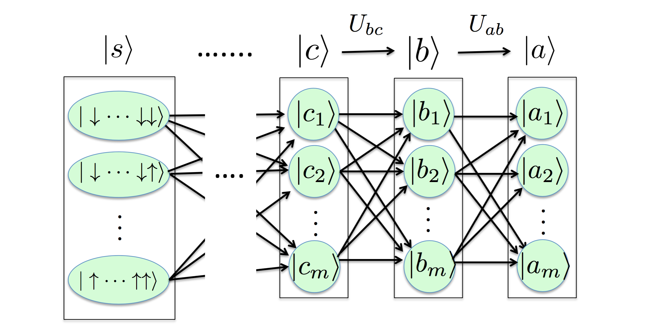
In DMRG we not only have "one-time" transformation, however. In the quantum mechanics (linear algebra) language (defining \(\sum_a \lvert a \rangle \langle a \lvert = I\)), an arbitrary state
\begin{equation*}
\lvert a \rangle = \Big( \sum_b \lvert b \rangle \langle b \lvert \Big) \lvert a\rangle = \sum_b \lvert b \rangle \langle b \lvert a \rangle = \sum_b \langle b \lvert a\rangle \lvert b \rangle = \sum_b U_{ab} \lvert b \rangle,
\end{equation*}
where
\( U_{ab}=\langle b \lvert a\rangle \) is the transformation matrix converting the base state
\( \lvert b\rangle \) to
\( \lvert a\rangle \), just like
\( U_{reduce} \). We can continue the above procedure and gain
\begin{equation*}
\lvert a \rangle = \sum_b U_{ab} \lvert b \rangle = \sum_b U_{ab} \Big( \sum_c \lvert c \rangle \langle c \lvert \Big) \lvert b \rangle = \sum_{b,c} U_{ab} U_{bc} \lvert c \rangle = \sum_{b,c,d} U_{ab} U_{bc} U_{cd} \lvert d \rangle = \cdots
\end{equation*}
In other words, the above equation tells us that
\( \lvert a\rangle \) is a linear combination of
\( \lvert b\rangle \),
\( \lvert b\rangle \) is a linear combination of
\( \lvert c\rangle \), and ....
until the
\( 2^D \) most primitive spin basis states
\( \lvert s \rangle = \) \( \lbrace \lvert \downarrow \downarrow \cdots \downarrow \rangle \cdots \lvert \uparrow \uparrow \cdots \uparrow \rangle \rbrace \). Hence any resulting states or wave functions can be obtained from iterative transformations on basis states. This is the renormalization process.
In this manner, it is analogous to neural network: nodes of the output layer are determined by those of the hidden layer, .. and nodes of the hidden layer are determined by those of the input layer. Therefore, the DMRG algorithm is analogous to the combination of PCA and neural network; each iteration or a transformation in DMRG is a layer representation in neural network. In addition to the DMRG, there is another renormalization process implementation proposed in deep learning (see the paper).